We help manufacturers & retailers to drive agility in supply chain execution
Pando's AI-powered, no-code & unified platform optimizes & automates your freight sourcing, transportation management, freight audit & payments

Pando is recognized by Gartner® in the 2024 International Context of Magic Quadrant™ for Transportation Management Systems

Pando named a Leader by G2
in the Spring 2024 Grid® Report
Based on high customer satisfaction score & having a large market presence in the Freight Management & Transporation Management Systems categories.

.svg)
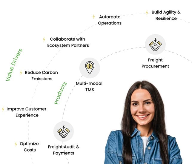
Freight Management

All Products
Transportation Management Systems


Freight
Procurement
Automate procurement with pre-defined templates, freight benchmarking, carrier discovery, scenario planning & manage dynamic contracts
Multi-modal
TMS
Optimized transportation planning with collaborative execution across modes, legs of movement driving real-time visibility
Freight Audit
& Payment
Unlock 100% freight spend visibility with flexible rate management, digital invoicing, automated reconciliation, accruals & payments
Automate procurement with pre-defined templates, freight benchmarking, carrier discovery, scenario planning & manage dynamic contracts
Optimized transportation planning with collaborative execution across modes, legs of movement driving real-time visibility
Unlock 100% freight spend visibility with flexible rate management, digital invoicing, automated reconciliation, accruals & payments
United teams fulfill dreams
Discover how your team can benefit from a modern, end-to-end unified Fulfillment Cloud.
Pando is loved by...
One touch integrations
Plug and play APIs to integrate seamlessly with enterprise ERPs, carrier systems, IoT devices, and other solutions in your business.
World-class security
Enterprise-grade platform with access rights management, data security, mobility, document management, and a data lake.
Effortless UX
Intuitive, network-first user experience that drives speedy adoption across your supply chain network.
Unified master data
Master data management across all your vendors, carriers, facilities, SKUs, and customers in one place.
Immediate ROI
Reduce freight costs by 12-14% within two quarters post-implementation.
Simplify freight audit & payment
Enable strict control over base and accessorial freight through our unified platform.
Currency & tax control
Unlock automatic currency conversion and global tax compliance for freight.
Better PO accuracy
Modular solutions backed by our powerful unified platform allow for better control for direct materials, inbound and outbound freight.
Simplify order coordination
Say goodbye to coordination between distribution center teams and customers for order visibility. You just need to send a magic link on dispatch!
Recognize revenue faster
Quicker dispatches and faster deliveries means shorter order-to-cash cycles.
Better customer service
Ensure real-time end-to-end visibility and ETA availability for customers.
Reliable deliveries with On-Time In-Full assurance
Improve service level adherence by 21% with streamlined order fulfillment.
Real-time visibility
Benefit from availability of shipment status and ETA from time of order until delivery.
Data-backed resolution across delivery issues
Time-stamp each activity from dispatch to delivery and enable closed loop availability of audit trail for all deliveries.
Real-time communication
Online communication of shipment creation, modifications, and spot RFQs for easy coordination with shipper.
Easy & accurate invoicing
Unlock access to automated rate calculations for each shipment that tie back to contracts.
Faster payments
Reduce payment cycles to less than 15 days from shipment execution.
Streamlined business
Digitization of all transactions removing human errors and inefficiencies.
Increased inclusivity into shipper's business
Enhance supplier collaboration from PO creation until delivery realization.
Simplify dispatch process
Provide real-time visibility to suppliers with regard to pickup schedules, carrier information, and driver details for coordinated handover.
Easy resolution across supply issues
Time-stamp each activity from pick up to delivery at shipper's location with a reliable audit trail.
IT

One touch integrations
Plug and play APIs to integrate seamlessly with enterprise ERPs, carrier systems, IoT devices, and other solutions in your business.
World-class security
Enterprise-grade platform with access rights management, data security, mobility, document management, and a data lake.
Effortless UX
Intuitive, network-first user experience that drives speedy adoption across your supply chain network.
Unified master data
Master data management across all your vendors, carriers, facilities, SKUs, and customers in one place.
Finance

Immediate ROI
Reduce freight costs by 12-14% within two quarters post-implementation.
Simplify freight audit & payment
Enable strict control over base and accessorial freight through our unified platform.
Currency & tax control
Unlock automatic currency conversion and global tax compliance for freight.
Better PO accuracy
Modular solutions backed by our powerful unified platform allow for better control for direct materials, inbound and outbound freight.
Sales

Simplify order coordination
Say goodbye to coordination between distribution center teams and customers for order visibility. You just need to send a magic link on dispatch!
Recognize revenue faster
Quicker dispatches and faster deliveries means shorter order-to-cash cycles.
Better customer service
Ensure real-time end-to-end visibility and ETA availability for customers.
Customers

Reliable deliveries with On-Time In-Full assurance
Improve service level adherence by 21% with streamlined order fulfillment.
Real-time visibility
Benefit from availability of shipment status and ETA from time of order until delivery.
Data-backed resolution across delivery issues
Time-stamp each activity from dispatch to delivery and enable closed loop availability of audit trail for all deliveries.
Carriers

Real-time communication
Online communication of shipment creation, modifications, and spot RFQs for easy coordination with shipper.
Easy & accurate invoicing
Unlock access to automated rate calculations for each shipment that tie back to contracts.
Faster payments
Reduce payment cycles to less than 15 days from shipment execution.
Streamlined business
Digitization of all transactions removing human errors and inefficiencies.
Suppliers

Increased inclusivity into shipper's business
Enhance supplier collaboration from PO creation until delivery realization.
Simplify dispatch process
Provide real-time visibility to suppliers with regard to pickup schedules, carrier information, and driver details for coordinated handover.
Easy resolution across supply issues
Time-stamp each activity from pick up to delivery at shipper's location with a reliable audit trail.
Your unique needs: Fulfilled
Explore how Pando's unified Fulfillment Cloud can help drive business impact for your industry.


Agile supply chains are powered by Pando


Congratulations to Pando for making their debut in the Gartner TMS Magic Quadrant! Our partnership with Pando has accelerated our visibility on ocean freight and improved rate management. Pando has helped us realize significant cost savings, deliver superior customer experience, and collaborate with our ecosystem partners seamlessly to build an agile supply chain. Pando gives us a competitive advantage in the marketplace!

Glad to witness Pando's recognition by Gartner! Through their integration of advanced AI technology, logistics expertise, and top-tier talent, Pando has become a key partner for us. Their solutions streamline our freight procurement to payment processes, driving meaningful changes in our supply chain toward greater agility and sustainability. Congratulations to the Pando team for their well-deserved recognition!

Congratulations to Pando on the well-deserved Gartner recognition! We needed a unified platform to collaborate with our vendors seamlessly, derive intelligence from our network, plug into our evolving IT landscape, scale with our business, and provide rapid value realization and Pando checked all our boxes. We're proud to be a Pando customer!

Pando's platform provides the end-to-end freight spend visibility, real-time analytics, predictive intelligence and collaborative automation through its AI tools, to optimize our logistics operations. These AI tools complement our supply chain team, so they are able to do more and have a greater impact than before!
Discover your path to supply chain agility. Speak to our experts today!
